ommx_pyscipopt_adapter

Submodules

• ommx_pyscipopt_adapter.adapter
• ommx_pyscipopt_adapter.exception

Exceptions

OMMXPySCIPOptAdapterError

Common base class for all non-exit exceptions.

Classes

OMMXPySCIPOptAdapter	Solve OMMX problems with SCIP through PySCIPOpt.
SCIPDiagnosticsAnalyzer	Pandas-like post-processor for PySCIPOpt diagnostics.
SCIPProgressSnapshot	SCIP solve progress observed during a solve.
SCIPTerminationReport	SCIP-side termination summary recorded after model.optimize().

Package Contents

exception OMMXPySCIPOptAdapterError

Common base class for all non-exit exceptions.

class OMMXPySCIPOptAdapter(ommx_instance: Instance, *, initial_state: ToState | NamedState | None = None)

Solve OMMX problems with SCIP through PySCIPOpt.

Install the ommx-pyscipopt-adapter package alongside a compatible OMMX SDK to use these examples. INPUT_CLASS defines the exact supported input. Nonconstant linear Indicator bodies and SOS1 constraints use SCIP's native addConsIndicator and addConsSOS1 operations. A nonconstant equality indicator becomes two inequality indicators. A constant body is simplified: a satisfied body needs no row, while an unsatisfied body forces its indicator to zero. OneHot constraints are lowered to regular equalities by the recommended preparation policy.

solve() prepares an isolated copy, leaving the caller's Instance unchanged. solve_without_preparation() and the constructor require the input to satisfy INPUT_CLASS already.

Build, solve, and inspect a 0-1 knapsack problem

Select items to maximize their total value while keeping their total weight at most the capacity. Each Binary variable is one when its item is selected. The names and subscripts preserve the connection to the input data:

>>> from ommx import Instance, Solution
>>> from ommx_pyscipopt_adapter import OMMXPySCIPOptAdapter
>>> values = [10, 13, 18, 31, 7, 15]
>>> weights = [11, 25, 20, 35, 10, 33]
>>> capacity = 47
>>> problem = Instance.maximize()
>>> items = [problem.new_binary("item", subscripts=[i]) for i in range(len(values))]
>>> problem.objective = sum(value * item for value, item in zip(values, items))
>>> weight_limit = problem.add_constraint(
...     sum(weight * item for weight, item in zip(weights, items)) <= capacity,
...     "Weight limit",
... )
>>> solution = OMMXPySCIPOptAdapter.solve(problem)
>>> assert solution.feasible
>>> assert solution.optimality == Solution.OPTIMAL
>>> selected = sorted(
...     i for (i,), value in solution.extract_decision_variables("item").items()
...     if value > 0.5
... )
>>> selected
[0, 3]
>>> assert abs(solution.objective - sum(values[i] for i in selected)) < 1e-6
>>> assert abs(solution.objective - 41.0) < 1e-6

ommx.Solution.objective is the returned candidate's objective value; the value alone does not establish optimality. Here SCIP proves optimality for the problem being evaluated. The decision-variable table provides IDs, names, subscripts, and values for tabular analysis. The regular-constraint table reports the normalized left-hand side: total weight minus capacity.

>>> variables = solution.decision_variables_df()
>>> assert set(variables["name"]) == {"item"}
>>> assert sorted(variables["value"]) == [0.0, 0.0, 0.0, 0.0, 1.0, 1.0]
>>> selection = variables[["subscripts", "value"]].copy()
>>> selection["choice"] = selection["value"].map(
...     lambda value: "Include" if value > 0.5 else "Exclude"
... )
>>> assert selection["choice"].value_counts().to_dict() == {"Exclude": 4, "Include": 2}
>>> constraints = solution.constraints_df(kind=ConstraintKind.Regular)
>>> residual = constraints.loc[weight_limit.constraint_id, "value"]
>>> assert abs(residual - (sum(weights[i] for i in selected) - capacity)) < 1e-6
>>> assert abs(residual - (-1.0)) < 1e-6

The selected items weigh 46, so the inequality has one unit of slack. ommx.Solution documents result extraction and evaluation semantics. The input can also come from a modeler, ommx.Instance.load_mps(), or ommx.artifact.Artifact; model construction is independent of solve.

Native Indicator and SOS1 constraints

This model rewards enabling a feature and selecting options. When enabled is one, the Indicator requires option_a + option_b <= 1. The SOS1 allows at most one of option_b and option_c to be nonzero; it does not require either one to be selected. SCIP receives both structures directly:

>>> from ommx import Instance, Sos1Constraint, ConstraintKind
>>> from ommx_pyscipopt_adapter import OMMXPySCIPOptAdapter
>>> source = Instance.maximize()
>>> enabled = source.new_binary("enabled")
>>> option_a = source.new_binary("option_a")
>>> option_b = source.new_binary("option_b")
>>> option_c = source.new_binary("option_c")
>>> source.objective = 10 * enabled + 6 * option_a + 5 * option_b + 4 * option_c
>>> _ = source.add_indicator_constraint((option_a + option_b <= 1).with_indicator(enabled))
>>> _ = source.add_sos1_constraint(
...     Sos1Constraint(variables=[option_b, option_c], name="exclusive_options")
... )
>>> assert OMMXPySCIPOptAdapter.INPUT_CLASS.contains(source)
>>> solution = OMMXPySCIPOptAdapter.solve(source)
>>> assert solution.feasible
>>> assert abs(solution.objective - 20.0) < 1e-6
>>> assert source.active_special_constraint_kinds == {
...     ConstraintKind.Indicator, ConstraintKind.Sos1,
... }
>>> assert not source.removed_constraints

The selected values are enabled = option_a = option_c = 1 and option_b = 0. The ommx_highs_adapter.OMMXHighsAdapter Reference solves this same model through lowering, demonstrating the distinction between native support and preparation for a target input class.

OneHot preparation without changing the source

Exactly one of the three binary variables must be one. The easy solve path lowers the OneHot constraint on its copy before encoding SCIP input:

>>> from ommx import Instance, OneHotConstraint, ConstraintKind
>>> from ommx_pyscipopt_adapter import OMMXPySCIPOptAdapter
>>> choice_model = Instance.maximize()
>>> choices = [choice_model.new_binary("choice", subscripts=[i]) for i in range(3)]
>>> choice_model.objective = 5 * choices[0] + 10 * choices[1] + 3 * choices[2]
>>> _ = choice_model.add_one_hot_constraint(OneHotConstraint(variables=choices))
>>> assert not OMMXPySCIPOptAdapter.INPUT_CLASS.contains(choice_model)
>>> solution = OMMXPySCIPOptAdapter.solve(choice_model)
>>> assert solution.feasible
>>> assert abs(solution.objective - 10.0) < 1e-6
>>> assert choice_model.active_special_constraint_kinds == {ConstraintKind.OneHot}
>>> assert not choice_model.removed_constraints

SOS1 with continuous variables

Native SOS1 support also applies to continuous variables: at most one may be nonzero, and all may be zero.

>>> from ommx import Instance, Sos1Constraint
>>> from ommx_pyscipopt_adapter import OMMXPySCIPOptAdapter
>>> sparse_model = Instance.maximize()
>>> ys = [sparse_model.new_continuous("y", lower=0, upper=10, subscripts=[i]) for i in range(3)]
>>> sparse_model.objective = sum(ys)
>>> _ = sparse_model.add_sos1_constraint(Sos1Constraint(variables=ys))
>>> solution = OMMXPySCIPOptAdapter.solve(sparse_model)
>>> assert solution.feasible
>>> assert abs(solution.objective - 10.0) < 1e-6

Select a policy and use the strict solve path

Here the application permits only OneHot lowering and keeps SOS1 native. Constructing the policy does not change the model. prepare changes the Instance in place and stops when the target class is reached; an enabled operation need not run if the input already belongs to that class.

>>> from ommx import (
...     Instance, OneHotConstraint, PreparationPolicy, Sos1Constraint,
...     ConstraintKind, SpecialConstraintPreparation,
... )
>>> from ommx_pyscipopt_adapter import OMMXPySCIPOptAdapter
>>> model = Instance.maximize()
>>> primary = [model.new_binary("primary", subscripts=[i]) for i in range(2)]
>>> optional = [model.new_binary("optional", subscripts=[i]) for i in range(2)]
>>> model.objective = 10 * primary[0] + 8 * primary[1] + 4 * optional[0] + 3 * optional[1]
>>> _ = model.add_one_hot_constraint(OneHotConstraint(variables=primary))
>>> _ = model.add_sos1_constraint(Sos1Constraint(variables=optional))
>>> policy = PreparationPolicy(
...     special_constraints=SpecialConstraintPreparation.lower_special_constraints(
...         kinds={ConstraintKind.OneHot}
...     )
... )
>>> model.prepare(OMMXPySCIPOptAdapter.INPUT_CLASS, policy)
>>> assert OMMXPySCIPOptAdapter.check_applicability(model).is_member
>>> assert model.active_special_constraint_kinds == {ConstraintKind.Sos1}
>>> solution = OMMXPySCIPOptAdapter.solve_without_preparation(model)
>>> assert solution.feasible
>>> assert abs(solution.objective - 14.0) < 1e-6
>>> assert len(solution.decision_variables_df()) == 4

The strict call applies no additional preparation. Calling solve instead obtains a fresh recommended policy; it does not reuse the local policy variable. A recommendation is an editable starting point, not a guarantee that every model can reach INPUT_CLASS.

classmethod check_applicability(ommx_instance: Instance) → InstanceClassMembershipReport

Check INPUT_CLASS membership without mutation.

decode(data: Model) → Solution

Convert optimized pyscipopt.Model and ommx.Instance to ommx.Solution.

This method is intended to be used if the model has been acquired with solver_input for further adjustment of the solver parameters, and separately optimizing the model.

Note that alterations to the model may make the decoding process incompatible -- decoding will only work if the model still describes effectively the same problem as the OMMX instance used to create the adapter.

Backend optimality is mapped through the instance's output-objective semantics. It remains unspecified when active-formulation optimality does not transport to that objective.

Examples

>>> from ommx_pyscipopt_adapter import OMMXPySCIPOptAdapter
>>> from ommx import Instance, DecisionVariable

>>> p = [10, 13, 18, 32, 7, 15]
>>> w = [11, 15, 20, 35, 10, 33]
>>> x = [DecisionVariable.binary(i) for i in range(6)]
>>> instance = Instance.from_components(
...     decision_variables=x,
...     objective=sum(p[i] * x[i] for i in range(6)),
...     constraints={0: sum(w[i] * x[i] for i in range(6)) <= 47},
...     sense=Sense.Maximize,
... )

>>> adapter = OMMXPySCIPOptAdapter(instance)
>>> model = adapter.solver_input
>>> # ... some modification of model's parameters
>>> model.optimize()

>>> solution = adapter.decode(model)
>>> solution.objective
42.0

decode_to_state(data: Model) → State

Create an ommx.State from an optimized PySCIPOpt Model.

SCIP's inforunbd status raises ommx.InfeasibleOrUnboundedDetected. The caller can retain this unresolved result or explicitly request further analysis. Decoding does not re-solve the model or change SCIP's reduction settings.

Examples

The following example shows how to solve an unconstrained linear optimization problem with `x1` as the objective function.

>>> from ommx_pyscipopt_adapter import OMMXPySCIPOptAdapter
>>> from ommx import Instance, DecisionVariable

>>> x1 = DecisionVariable.integer(1, lower=0, upper=5)
>>> ommx_instance = Instance.from_components(
...     decision_variables=[x1],
...     objective=x1,
...     constraints={},
...     sense=Sense.Minimize,
... )
>>> adapter = OMMXPySCIPOptAdapter(ommx_instance)
>>> model = adapter.solver_input
>>> model.optimize()

>>> ommx_state = adapter.decode_to_state(model)
>>> ommx_state.entries
{1: 0.0}

classmethod recommended_preparation_policy() → PreparationPolicy

Recommend lowering OneHot constraints before using PySCIPOpt.

PySCIPOpt accepts Indicator and SOS1 constraints directly, so this recommendation preserves those families and lowers only OneHot constraints. The easy API applies a fresh policy to an isolated copy; callers may instead edit and apply one before invoking solve_without_preparation().

classmethod require_applicable(ommx_instance: Instance) → InstanceClassMembershipReport

Return the membership report or raise AdapterNotApplicableError.

classmethod solve(ommx_instance: Instance, *, initial_state: ToState | NamedState | None = None, diagnostics: DiagnosticsSink | None = None) → Solution

Solve the given ommx.Instance using PySCIPopt, returning an ommx.Solution.

The input instance is not modified. An isolated copy is prepared with the recommended PySCIPOpt policy before preparation-free execution.

パラメータ:

• ommx_instance -- The ommx.Instance to prepare and solve.

• initial_state -- Optional initial solution as a State, ID-keyed values, or values grouped by name and tuple subscripts.

Examples

The OMMXPySCIPOptAdapter class documentation contains a complete knapsack example from model construction through named-variable extraction, tabular analysis, objective value, and constraint slack.

Start from a candidate

Evaluate the proposed assignment against the same instance you intend to solve. SCIP uses it as a starting point and can return a better solution. In this example the starting objective is 1 and the optimum is 5.

>>> from ommx import Instance
>>> from ommx_pyscipopt_adapter import OMMXPySCIPOptAdapter
>>> problem = Instance.maximize()
>>> x = problem.new_integer("x", lower=0, upper=5)
>>> y = problem.new_integer("y", lower=0, upper=5)
>>> problem.objective = x - y
>>> _ = problem.add_constraint(x + y <= 5)
>>> proposed = {x.id: 3, y.id: 2}
>>> initial = problem.evaluate(proposed)
>>> assert initial.feasible and initial.objective == 1
>>> result = OMMXPySCIPOptAdapter.solve(problem, initial_state=proposed)
>>> assert result.feasible and result.objective == 5

To reuse a plan across models whose IDs differ, supply names and tuple subscripts. Use an empty tuple for a scalar and (i,) for a single index. SCIP accepts the named mapping directly. To check it first, resolve the names against the target instance:

>>> named = {"x": {(): 3.0}, "y": {(): 2.0}}
>>> state = problem.state_from_named_values(named)
>>> assert problem.evaluate(state).feasible
>>> assert OMMXPySCIPOptAdapter.solve(problem, initial_state=named).objective == 5

You can also pass the resolved State or a previous solution's state when the IDs match. ommx.Instance.state_from_named_values() describes unknown or ambiguous names. SCIP initializes omitted solver variables to zero when building the proposed solution. Evaluating a partial assignment with OMMX may require additional values. A starting point neither fixes the final assignment nor guarantees a shorter solve.

Infeasible Problem

>>> from ommx import Instance, DecisionVariable, Sense
>>> from ommx_pyscipopt_adapter import OMMXPySCIPOptAdapter

>>> x = DecisionVariable.integer(0, upper=3, lower=0)
>>> instance = Instance.from_components(
...     decision_variables=[x],
...     objective=x,
...     constraints={0: x >= 4},
...     sense=Sense.Maximize,
... )

>>> OMMXPySCIPOptAdapter.solve(instance)
Traceback (most recent call last):
    ...
ommx.InfeasibleDetected: Model was infeasible

Unbounded Problem

>>> from ommx import Instance, DecisionVariable, Sense
>>> from ommx_pyscipopt_adapter import OMMXPySCIPOptAdapter

>>> x = DecisionVariable.integer(0, lower=0)
>>> instance = Instance.from_components(
...     decision_variables=[x],
...     objective=x,
...     constraints={},
...     sense=Sense.Maximize,
... )

>>> OMMXPySCIPOptAdapter.solve(instance)
Traceback (most recent call last):
    ...
ommx.adapter.UnboundedDetected: Model was unbounded

classmethod solve_without_preparation(ommx_instance: Instance, *, initial_state: ToState | NamedState | None = None, diagnostics: DiagnosticsSink | None = None) → Solution

Solve an exact PySCIPOpt Adapter input without preparing it.

INPUT_CLASS: ClassVar[InstanceClass]

Required condition for an exact Adapter input.

property solver_input: Model

The PySCIPOpt model generated from this OMMX instance

class SCIPDiagnosticsAnalyzer(diagnostics: Iterable[Any])

Pandas-like post-processor for PySCIPOpt diagnostics.

Inspect why SCIP stopped and how its search progressed. A Solution evaluates a candidate against the OMMX problem; diagnostics report what the backend observed or proved about the formulation it solved. A feasible candidate alone does not establish optimality.

Collect a final report

Install the SDK and PySCIPOpt Adapter using the installation guide. This example builds a small binary problem: choose at most one item and maximize its value. It needs neither an external dataset nor an Experiment.

>>> from ommx import Instance
>>> from ommx.adapter import DiagnosticCollector
>>> from ommx_pyscipopt_adapter import OMMXPySCIPOptAdapter, SCIPDiagnosticsAnalyzer
>>> instance = Instance.maximize()
>>> x = instance.new_binary("x")
>>> y = instance.new_binary("y")
>>> instance.objective = 3 * x + 2 * y
>>> _ = instance.add_constraint(x + y <= 1)
>>> collector = DiagnosticCollector()
>>> solution = OMMXPySCIPOptAdapter.solve(instance, diagnostics=collector)
>>> analysis = SCIPDiagnosticsAnalyzer(collector.diagnostics)
>>> solution.objective, solution.feasible
(3.0, True)
>>> solution.decision_variables_df()[["name", "value"]].to_dict("records")
[{'name': 'x', 'value': 1.0}, {'name': 'y', 'value': 0.0}]
>>> result = analysis.termination_result
>>> assert result is not None
>>> result["status"], result["primal_bound"], result["dual_bound"], result["gap"]
('optimal', 3.0, 3.0, 0.0)

The candidate selects x=1, y=0. status == "optimal" is SCIP's final optimality report; it is distinct from OMMX's feasibility check. A time-limited solve can return a feasible candidate without proving optimality.

primal_bound is the best feasible objective bound found by the solver; dual_bound bounds how good the optimum can still be. For maximization, the primal bound is a lower bound and the dual bound an upper bound; their roles as upper/lower bounds reverse for minimization. gap is SCIP's reported relative gap, not simply their arithmetic difference. Bounds and gaps need not be finite when, for example, no candidate has been found. SCIP may also represent infinity by a large finite sentinel.

These values concern the solver-facing objective. After sign, scale, or penalty changes, do not treat them as bounds on the reported OMMX objective without the corresponding transformation guarantee. See result interpretation.

Read progress observations

The analyzer accepts either typed diagnostics collected by ommx.adapter.DiagnosticCollector or dictionaries loaded from ommx.experiment.Solve.diagnostics.

progress_history_records returns list[dict[str, object]] and does not require pandas. When diagnostics include a terminal SCIP report, the progress history includes a final TERMINATION row derived from that report. progress_history_df returns a pandas DataFrame indexed by solving_time_sec and imports pandas lazily. Time-series properties such as dual_bound return pandas Series with the same index. termination_result returns the terminal SCIP report as a dictionary.

>>> history = analysis.progress_history_df
>>> history.index.name
'solving_time_sec'
>>> history.iloc[-1]["event"]
'TERMINATION'
>>> float(analysis.dual_bound.iloc[-1]), float(analysis.gap.iloc[-1])
(3.0, 0.0)
>>> assert analysis.incumbent_objective.iloc[-1] == solution.objective
>>> assert analysis.progress_history_records[-1]["event"] == "TERMINATION"

Small problems may have few intermediate points. SCIP records SCIPProgressSnapshot at BESTSOLFOUND and DUALBOUNDIMPROVED callbacks, plus a final TERMINATION snapshot. Callbacks can run before aggregate statistics are updated; read terminal values from the final row or SCIPTerminationReport. The report also includes node/LP/cut counters, primal-dual integral, timings, and solver version metadata.

Plot a recorded bound and gap history

Use the elapsed-time index to plot the bounds and gap from your own run. SCIP can return its infinity sentinel before a finite bound is available. Mask these entries so an unknown bound does not look like a large observed value.

>>> from matplotlib import pyplot as plt
>>> from pyscipopt import Model
>>> values = history[["primal_bound", "dual_bound", "gap"]].astype(float)
>>> visible = values.where(values.abs() < Model().infinity())
>>> fig, (bounds_ax, gap_ax) = plt.subplots(2, sharex=True)
>>> _ = visible[["primal_bound", "dual_bound"]].plot(ax=bounds_ax)
>>> _ = visible["gap"].plot(ax=gap_ax, ylabel="Relative gap")
>>> plt.close(fig)

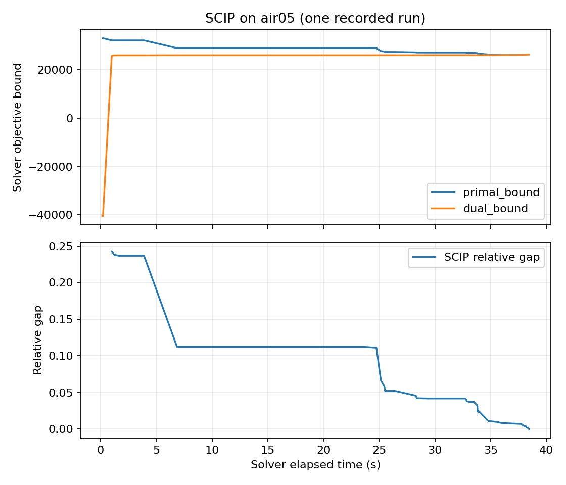
SCIP 10.0.2 minimizing MIPLIB air05 with the adapter defaults. The incumbent gives an upper bound and the dual bound gives a lower bound. Lines connect recorded observations. At termination the bounds meet at 26,374 and SCIP reports a relative gap of zero.

Inspect a report when no Solution is returned

The Adapter records termination before decoding the solver result. If decoding raises an adapter exception, the collector can therefore retain the final report. This unbounded problem has no finite optimum:

>>> from ommx.adapter import UnboundedDetected
>>> unbounded = Instance.maximize()
>>> z = unbounded.new_continuous("z", lower=0)
>>> unbounded.objective = z
>>> collector = DiagnosticCollector()
>>> try:
...     OMMXPySCIPOptAdapter.solve(unbounded, diagnostics=collector)
... except UnboundedDetected:
...     failure = SCIPDiagnosticsAnalyzer(collector.diagnostics).termination_result
>>> assert failure is not None and failure["status"] == "unbounded"

Errors before the backend finishes need not produce a termination report; termination_result is None when no such report was collected.

Read diagnostics saved with an Experiment

Recording is optional. log_solve() owns the diagnostics keyword; pass store_diagnostics=True instead of a collector. Collection is disabled by default. The following example uses the small model above and a temporary Local Registry.

>>> from ommx.experiment import Experiment
>>> with Experiment.with_temp_local_registry() as experiment:
...     with experiment.run() as run:
...         solution = run.log_solve(
...             OMMXPySCIPOptAdapter, instance, store_diagnostics=True,
...         )
>>> stored = experiment.runs[0].solves[0].diagnostics
>>> assert stored and all(isinstance(report, dict) for report in stored)
>>> saved = SCIPDiagnosticsAnalyzer(stored)
>>> assert saved.termination_result["status"] == "optimal"
>>> assert saved.dual_bound.iloc[-1] == 3.0

Stored reports are dictionaries rather than the original Python dataclasses. Both forms support the same records, DataFrame, and Series views. If an Adapter raises, log_solve records a failed/interrupted Solve without an output Solution when possible, including diagnostics collected before the failure. log_sample() records sampling outcomes separately. Persistence is best-effort; consult those methods for failure handling and the reserved keyword contract.

property dual_bound: Any

Return dual bounds indexed by solving time.

property event: Any

Return progress event names indexed by solving time.

property gap: Any

Return relative gaps indexed by solving time.

property incumbent_objective: Any

Return incumbent objectives indexed by solving time.

property lp_iteration_count: Any

Return LP iteration counts indexed by solving time.

property node_count: Any

Return processed node counts indexed by solving time.

property primal_bound: Any

Return primal bounds indexed by solving time.

property progress_history_df: Any

Return progress history as a pandas DataFrame indexed by time.

property progress_history_records: list[dict[str, object]]

Return SCIP progress history, with TERMINATION when present.

property progress_snapshots: tuple[SCIPProgressSnapshot, ...]

Typed progress snapshots in the order they were recorded.

property solution_count: Any

Return stored solution counts indexed by solving time.

property termination_result: dict[str, object] | None

Return the terminal SCIP report as one dictionary, if present.

property total_node_count: Any

Return total processed node counts indexed by solving time.

class SCIPProgressSnapshot

SCIP solve progress observed during a solve.

The PySCIPOpt adapter records this snapshot for each tracked SCIP event and once more from the termination report after model.optimize() finishes. It currently listens for BESTSOLFOUND and DUALBOUNDIMPROVED. Event snapshots are the model state visible from that callback. SCIP may call a BESTSOLFOUND callback before every aggregate model statistic has been updated, so use the TERMINATION snapshot or SCIPTerminationReport for terminal values.

classmethod from_event(model: Model, event: Event) → SCIPProgressSnapshot

classmethod from_termination_report(report: SCIPTerminationReport) → SCIPProgressSnapshot

dual_bound: float

SCIP dual bound reported at the snapshot.

event: str

Progress marker.

Callback snapshots use SCIP event names such as "BESTSOLFOUND" and "DUALBOUNDIMPROVED". The terminal snapshot uses the synthetic "TERMINATION" marker.

gap: float

SCIP relative gap reported at the snapshot.

incumbent_objective: float | None

Objective value of SCIP's current best solution.

This is None when PySCIPOpt cannot read an incumbent objective at that snapshot.

lp_iteration_count: int

LP iterations at the snapshot.

node_count: int

Processed branch-and-bound nodes at the snapshot.

primal_bound: float

SCIP primal bound reported at the snapshot.

solution_count: int

Number of solutions stored by SCIP at the snapshot.

solving_time_sec: float

SCIP solving time when the snapshot was recorded.

total_node_count: int

Total processed nodes including restarts at the snapshot.

class SCIPTerminationReport

SCIP-side termination summary recorded after model.optimize().

The PySCIPOpt adapter records this report before decoding the optimized SCIP model back into an OMMX solution. It is therefore available even when decoding raises an adapter exception such as infeasible or unbounded detection.

classmethod from_model(model: Model) → SCIPTerminationReport

applied_cut_count: int

Number of cuts applied by SCIP.

best_solution_count: int

Number of new incumbent solutions SCIP found.

cut_count: int

Number of cuts available in SCIP's cut pool.

dual_bound: float

SCIP dual bound at termination.

gap: float

SCIP relative gap reported by getGap().

lp_iteration_count: int

Total LP iterations.

lp_solve_count: int

Number of solved LPs.

max_depth: int

Maximum branch-and-bound depth.

SCIP may report -1 when no branching occurred.

node_count: int

Number of branch-and-bound nodes processed by SCIP.

objective_value: float | None

Incumbent objective value, or None when SCIP has no solution.

presolving_time_sec: float

SCIP presolving time in seconds.

primal_bound: float

SCIP primal bound at termination.

primal_dual_integral: float

SCIP primal-dual integral at termination.

pyscipopt_version: str | None

PySCIPOpt package version, if available.

reading_time_sec: float

SCIP reading time in seconds.

scip_version: str

SCIP version used through PySCIPOpt.

solution_count: int

Number of solutions stored by SCIP at termination.

solution_found_count: int

Number of solutions SCIP found during the solve.

solving_time_sec: float

SCIP solving time in seconds.

status: str

SCIP termination status, such as "optimal", "infeasible", or "unbounded".

total_node_count: int

Total processed nodes including restarts.