Sampling from QUBO with OMMX Adapter

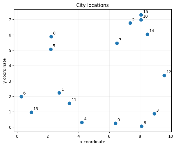
This tutorial uses the Traveling Salesman Problem (TSP) to show the complete workflow from an OMMX model to samples returned by OpenJij. The city layout and the sampled route are plotted so that the result can be inspected directly.

TSP asks for the shortest route that visits every city exactly once and returns to the starting city. We generate 16 cities in a 10 by 10 region with a fixed random seed, making the example reproducible.

from random import Random

CITY_COUNT = 16
random = Random(42)
city_points = [
    (random.uniform(0.0, 10.0), random.uniform(0.0, 10.0))
    for _ in range(CITY_COUNT)
]

%matplotlib inline
from matplotlib import pyplot as plt

fig, ax = plt.subplots(figsize=(7, 7))
city_x, city_y = zip(*city_points)
ax.scatter(city_x, city_y, s=60)
for city, point in enumerate(city_points):
    ax.annotate(str(city), point, xytext=(5, 5), textcoords="offset points")
ax.set(
    title="City locations",
    xlabel="x coordinate",
    ylabel="y coordinate",
)
ax.set_aspect("equal", adjustable="box")
ax.grid(alpha=0.2)
plt.show()

Let \(d(i, j)\) be the Euclidean distance between cities \(i\) and \(j\).

def distance(left: tuple[float, float], right: tuple[float, float]) -> float:
    return ((left[0] - right[0]) ** 2 + (left[1] - right[1]) ** 2) ** 0.5


distances = [
    [distance(city_points[i], city_points[j]) for j in range(CITY_COUNT)]
    for i in range(CITY_COUNT)
]

We use a Binary decision variable \(x_{t,i}\) that is one when city \(i\) is visited at position \(t\) in the route. The objective is the length of the closed route:

\[ \sum_{t=0}^{N-1} \sum_{i,j=0}^{N-1} d(i,j)x_{t,i}x_{(t+1) \bmod N,j}. \]

At each position exactly one city must be selected, and every city must appear exactly once:

\[ \sum_{i=0}^{N-1}x_{t,i}=1 \quad (\forall t), \qquad \sum_{t=0}^{N-1}x_{t,i}=1 \quad (\forall i). \]

The names and subscripts attached to the decision variables are retained by OMMX and will later let us reconstruct a route from a sample.

from ommx import DecisionVariable, Instance, Sense

route_variables = [
    [
        DecisionVariable.binary(
            city + CITY_COUNT * position,
            name="x",
            subscripts=[position, city],
        )
        for city in range(CITY_COUNT)
    ]
    for position in range(CITY_COUNT)
]

objective = sum(
    distances[i][j]
    * route_variables[position][i]
    * route_variables[(position + 1) % CITY_COUNT][j]
    for position in range(CITY_COUNT)
    for i in range(CITY_COUNT)
    for j in range(CITY_COUNT)
)

position_constraints = {
    position: (
        sum(route_variables[position][city] for city in range(CITY_COUNT)) == 1
    )
    .set_name("position")
    .add_subscripts([position])
    for position in range(CITY_COUNT)
}
city_constraints = {
    CITY_COUNT + city: (
        sum(route_variables[position][city] for position in range(CITY_COUNT))
        == 1
    )
    .set_name("city")
    .add_subscripts([city])
    for city in range(CITY_COUNT)
}

instance = Instance.from_components(
    decision_variables=[
        route_variables[position][city]
        for position in range(CITY_COUNT)
        for city in range(CITY_COUNT)
    ],
    objective=objective,
    constraints={**position_constraints, **city_constraints},
    sense=Sense.Minimize,
)

Sampling with OpenJij

from ommx import FixedPenaltyPreparation
from ommx_openjij_adapter import OMMXOpenJijSAAdapter

input_class = OMMXOpenJijSAAdapter.INPUT_CLASS

# Start from the model conversions recommended for OpenJij.
policy = OMMXOpenJijSAAdapter.recommended_preparation_policy()

# The penalty magnitude is application-specific, so the caller chooses it.
policy.fixed_penalty = (
    FixedPenaltyPreparation.uniform_penalty_method_with_fixed_weight(
        weight=10.0,
    )
)
instance.prepare(input_class, policy)

# Leave seed unset so each read can follow a different random trajectory.
sample_set = OMMXOpenJijSAAdapter.sample_without_preparation(
    instance,
    num_reads=32,
    num_sweeps=2000,
)

Instance conversion policy

OpenJij directly accepts unconstrained Binary minimization models. The TSP model has constraints and a penalty magnitude has no safe universal default, so we customize the Adapter’s recommended conversion policy and call prepare() on the Instance. The recommendation enables the conversions OpenJij commonly needs: lowering special constraints, normalizing the optimization sense, adding Integer slack, and encoding Integer variables.

Removing constraints requires a fixed penalty. Its magnitude is an OMMX model conversion setting, not an OpenJij sampler parameter, and there is no safe value for every model. A larger value encourages feasible samples but no finite value guarantees them.

For this generated instance, we use 10.0 as a starting point because its largest edge cost is about 9.5. This is a scale heuristic, not a formula for a sufficient penalty. Check both feasibility and sample diversity, then adjust the value for your model. Sampling is stochastic, so rerunning this notebook may produce different routes.

prepare() updates instance in place. If a later conversion fails, changes from earlier completed conversions remain on instance. The subsequent preparation-free sample_without_preparation() call checks that the Instance is an exact OpenJij input.

Viewing the results

summary = sample_set.summary
summary.head(10)

	objective	feasible
sample_id
4	68.945319	True
20	77.559905	True
18	77.908902	True
9	78.543482	True
23	79.505363	True
0	80.491507	True
12	81.954426	True
22	81.954426	True
30	81.954426	True
7	81.954426	True

SampleSet.summary is a pandas DataFrame containing the objective value and feasibility of each sample. OMMX retains the constraints removed during preparation, so feasible still tells us whether each sample satisfies the TSP constraints. objective is the original route length for every row; the fixed penalty affects OpenJij’s sampling energy but is not included in this column. The table is sorted with feasible samples first and then by objective value.

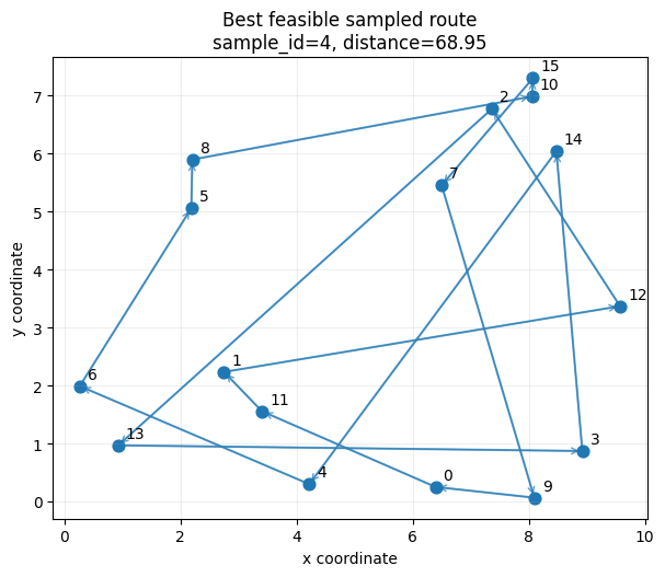
The registered variable name and subscripts let us extract \(x_{t,i}\) for a sample and turn it back into a route. Here we select the best feasible sample shown in the summary.

def sample_to_route(sample: dict[tuple[int, ...], float]) -> list[int]:
    return [
        next(
            city
            for city in range(CITY_COUNT)
            if sample[(position, city)] > 0.5
        )
        for position in range(CITY_COUNT)
    ]


if not sample_set.feasible_ids():
    raise RuntimeError(
        "No feasible route was sampled; try more reads or revisit the penalty."
    )

best_sample_id = sample_set.best_feasible_id
best_objective = sample_set.objectives[best_sample_id]
best_sample = sample_set.extract_decision_variables("x", best_sample_id)
sampled_route = sample_to_route(best_sample)
sampled_route

[9, 0, 11, 1, 12, 2, 13, 3, 14, 4, 6, 5, 8, 10, 15, 7]

route_cycle = sampled_route + [sampled_route[0]]

fig, ax = plt.subplots(figsize=(7, 7))
route_x = [city_points[city][0] for city in route_cycle]
route_y = [city_points[city][1] for city in route_cycle]
ax.plot(route_x, route_y, color="tab:blue", alpha=0.6)
ax.scatter(city_x, city_y, s=60, color="tab:blue")

for start, end in zip(route_cycle, route_cycle[1:]):
    ax.annotate(
        "",
        xy=city_points[end],
        xytext=city_points[start],
        arrowprops={"arrowstyle": "->", "color": "tab:blue", "alpha": 0.7},
    )
for city, point in enumerate(city_points):
    ax.annotate(str(city), point, xytext=(5, 5), textcoords="offset points")

ax.set(
    title=(
        f"Best feasible sampled route\n"
        f"sample_id={best_sample_id}, distance={best_objective:.2f}"
    ),
    xlabel="x coordinate",
    ylabel="y coordinate",
)
ax.set_aspect("equal", adjustable="box")
ax.grid(alpha=0.2)
plt.show()